Chapter 2: Data Overview

The dataset from the Kaggle challenge is organized as follows:

• Training Set: Contains 250,000 events with multiple features.
• Feature Columns: 30 feature columns, an ID column, a weight column, and a label column.

Key features include:

• All variables are in floating-point format, with the exception of PRI_jet_num, which is an integer.
• Variables prefixed with PRI (for PRImitives) represent raw measurements from the detector.
• Variables prefixed with DER (for DERived) are calculated features derived from the primitive measurements.
• Some entries may have missing values represented as ?999.0, which lies outside the expected range.

Chapter 3: Data Integration

To begin analyzing the data, I utilized the Kaggle notebook available at the following link:

Higgs

Explore and run machine learning code with Kaggle Notebooks | Using data from Higgs Boson Machine Learning Challenge

www.kaggle.com

Initially, I loaded the dataset into a pandas DataFrame with the following command:

data = pd.read_csv('../input/higgs-boson/training.zip')

Next, I removed two non-essential columns from the DataFrame:

df_data = data.drop(columns=['EventId', 'Weight'])

I then created two DataFrames: df for training and df_val for validation, where df_val holds unseen data to evaluate the model's performance.

from sklearn.model_selection import train_test_split

df, df_val = train_test_split(df_data, test_size=0.33, random_state=42)

Chapter 4: Train-Test Split

With df prepared, I proceeded with the train-test split. The label was extracted as the target variable, while the remaining columns were designated as features.

X = df.drop(columns=['Label']) # Features

y = df['Label'] # Target

The data was then divided into training and testing subsets (80% for training, 20% for testing):

X_train, X_test, y_train, y_test = train_test_split(X, y, test_size=0.2, random_state=42)

Subsequently, I constructed a voting classifier using ensemble methods:

from lightgbm import LGBMClassifier

from sklearn.ensemble import RandomForestClassifier, VotingClassifier

from sklearn.linear_model import LogisticRegression

from sklearn.metrics import accuracy_score

# Define classifiers

logistic_classifier = LogisticRegression()

rf_classifier = RandomForestClassifier()

lgbm_classifier = LGBMClassifier()

# Create a Voting Classifier

voting_classifier = VotingClassifier(estimators=[

('logistic', logistic_classifier),

('random_forest', rf_classifier),

('lgbm', lgbm_classifier)

], voting='soft')

# Train the classifier

voting_classifier.fit(X_train, y_train)

# Predictions

y_pred = voting_classifier.predict(X_test)

accuracy = accuracy_score(y_test, y_pred)

print(f"Accuracy: {accuracy:.2f}")

The model achieved an accuracy of 84%.

Chapter 5: Model Validation

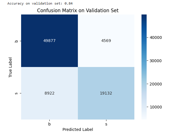
For validation, I utilized the saved model to predict labels for the validation set and generated a confusion matrix:

X_val = df_val.drop(columns=['Label']) # Features for df_val

y_val_true = df_val['Label'] # True target for df_val

y_val_pred = voting_classifier.predict(X_val)

accuracy_val = accuracy_score(y_val_true, y_val_pred)

print(f"Accuracy on validation set: {accuracy_val:.2f}")

To visualize the performance, I plotted the confusion matrix using Seaborn:

import seaborn as sns

import matplotlib.pyplot as plt

conf_matrix = confusion_matrix(y_val_true, y_val_pred)

sns.heatmap(conf_matrix, annot=True, fmt='d', cmap='Blues')

plt.title("Confusion Matrix on Validation Set")

plt.xlabel("Predicted Label")

plt.ylabel("True Label")

plt.show()

Chapter 6: Advanced Metrics

Finally, we can assess the sensitivity and specificity of the model. The algorithm effectively identifies the signal 68% of the time, demonstrating its utility in distinguishing the Higgs boson signal from background noise.

The first video, "Deep Learning for Higgs Boson Identification and Searches for New Physics," provides insights into advanced machine learning techniques used in particle physics.

The second video, "Higgs Boson: How do you search for it?" explores methodologies for identifying the Higgs boson in various experimental contexts.