Understanding Probability Distributions and Their Applications
Written on
Chapter 1: Overview of Probability Distributions
In this segment of our exploration into statistics with Python, we will delve into various types of probability distributions and their real-world applications. We will begin by examining the key variables associated with common probability distributions.

Common Probability Distribution
A probability distribution represents the likelihood of different outcomes for a random variable. A random variable denotes an uncertain outcome, such as the weather.
- Discrete Random Variables: These can only take on a limited number of specific values (e.g., whether it rains or not).
- Continuous Random Variables: These can assume an infinite number of values (e.g., stock returns).
Discrete Uniform Distribution
A discrete uniform distribution is characterized by a finite set of outcomes where each outcome has an equal chance of occurring. A classic example is rolling a six-sided die, where each face has a probability of 1/6.
Two properties define a discrete uniform distribution: - Probabilities range from 0 to 1. - The total of all probabilities equals 1.
Continuous Uniform Distribution
In contrast, a continuous uniform distribution has a density function and allows for an infinite number of outcomes, yet still maintains equal probability across those outcomes.
Joint Probabilities
Joint probabilities involve the likelihood of multiple events occurring, which can be mutually exclusive (e.g., it either rains or is sunny), concurrent (e.g., raining and sunny simultaneously), or non-mutually exclusive (e.g., it’s raining and an umbrella is needed).
Mutually Exclusive Events
For example, if the weather has four potential outcomes with equal probabilities (25% each: raining, drizzling, cloudy, sunny), we can calculate the joint probability of it being either drizzling or sunny.
p(drizzling or sunny) = 0.25 + 0.25 = 0.50 (or 50% chance).
Concurrent Occurring Events
If we want to assess the chance of it being both rainy and sunny, we multiply their probabilities:
p(rain and sunny) = 0.25 * 0.25 = 0.0625 (or 6.25% chance).
Non-Mutually Exclusive Events
For cases where we want to know the probability of either raining or needing an umbrella, assuming a 50% chance of needing an umbrella, we calculate:
p(rain or umbrella) = 0.25 + 0.50 = 0.75.
Then, we need to subtract the probability of both raining and needing an umbrella:
p(rain and umbrella) = 0.25 * 0.50 = 0.125.
Thus, the probability of it either raining or needing an umbrella is:
p(rain or umbrella) - p(rain and umbrella) = 0.75 - 0.125 = 0.625 (or 62.5%).
Binomial Distribution
A binomial distribution pertains to scenarios with two possible outcomes, such as flipping a coin, which can land on heads or tails.
Key assumptions include: - Each trial is independent. - The probability of success is consistent across trials.
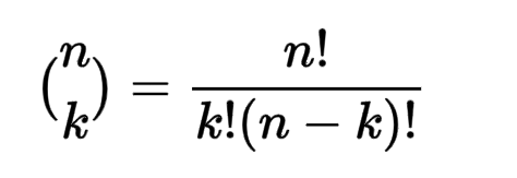
For example, to find the probability of a coin landing on heads twice in ten flips, we determine the number of combinations of getting two heads.

The binomial coefficient is calculated as follows:
= 10!/((10–2)!*2!) = 45.
Next, we compute the probability of getting two heads in ten flips using the binomial distribution formula:

The final probability of flipping two heads in ten tries is approximately 4.4%.
We can achieve this calculation efficiently using Python:
from scipy import stats # stats.binom.pmf(x,y,z) x = stats.binom.pmf(2,10,0.5) print(x) # 0.044
Where: - x = number of successes - y = number of trials - z = probability of success
Normal Distribution
A normal distribution is represented by a bell curve, characterized by specific features:

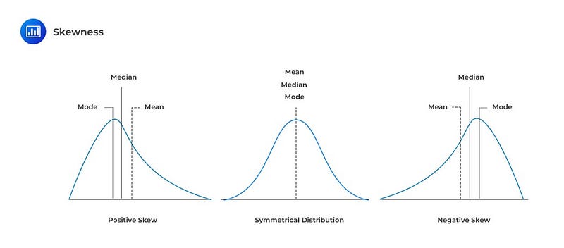
Distinct characteristics include: - Zero skewness. - Equality of mean, median, and mode. - Described through mean, variance, or standard deviation. - Kurtosis of three.
Approximately: - 50% of values lie within two-thirds of a standard deviation from the mean. - About 68% of values fall within one standard deviation. - Roughly 95% of values are within two standard deviations. - Approximately 99% lie within three standard deviations.
That concludes our third part in this series. I hope you now have a clearer understanding of various distributions and how to compute the probabilities of different events.
Stay tuned for Part 4!
This video serves as an introduction to Python programming, showcasing fundamental concepts and applications.
This video provides a deeper insight into statistics using Python, focusing on key principles and techniques.