Chapter 1: Understanding RMSprop

Root Mean Square Propagation, commonly known as RMSprop, is a sophisticated optimization technique that adjusts the learning rate dynamically, addressing certain drawbacks associated with ADAGRAD. Similar to ADAGRAD, RMSprop customizes the learning rate for each parameter, but it innovatively modifies the approach to prevent excessive reduction of the learning rate.

To maintain a more stable learning rate throughout the training process, RMSprop utilizes an exponentially decaying average of squared gradients. This adaptation allows for a consistent learning rate over multiple iterations. Let's delve into the contrasts between ADAGRAD and RMSprop:

? ADAGRAD continually sums the squared gradients:

This accumulation results in a progressive decrease in the learning rate, as the total of squared gradients increases, potentially leading to a minuscule learning rate over time.

? In contrast, RMSprop employs an exponentially weighted average of squared gradients:

This mechanism emphasizes recent gradients more heavily, thereby preventing a rapid decline in the learning rate. The learning rate is modified based on this moving average of squared gradients:

The moving average ensures a more gradual and controlled adjustment to the learning rate, fostering stability and reducing the likelihood of rapid decreases.

To clarify, let’s explore the concept of the exponentially-weighted moving average (EWMA). EWMA applies progressively diminishing weights to past data points, giving greater significance to more recent observations. An example can be illustrated through the following formulas:

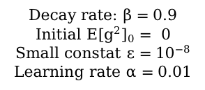
Given the following conditions:

In the first time step:

And in the second time step:

Let's illustrate this with a coding example!

First, we will define the function alongside its gradient:

import numpy as np

import matplotlib.pyplot as plt

# Define the function

def f(x, y):

return x ** 2 + 0.5 * y ** 2

# Gradient of the function

def gradient_f(x, y):

grad_x = 2 * x

grad_y = 0.2 * y

return grad_x, grad_y

Next, we will implement ADAGRAD for comparison, observing the number of iterations needed for both ADAGRAD and RMSprop:

# ADAGRAD function

def adagrad(eta, num_iterations, initial_x, initial_y):

x = initial_x

y = initial_y

eps = 1e-8 # small constant to avoid division by zero

sum_sq_gradients_x = 0

sum_sq_gradients_y = 0

x_values = [x]

y_values = [y]

for t in range(1, num_iterations + 1):

gradient_x, gradient_y = gradient_f(x, y)

sum_sq_gradients_x += gradient_x ** 2

sum_sq_gradients_y += gradient_y ** 2

adjusted_eta_x = eta / (np.sqrt(sum_sq_gradients_x) + eps)

adjusted_eta_y = eta / (np.sqrt(sum_sq_gradients_y) + eps)

x = x - adjusted_eta_x * gradient_x

y = y - adjusted_eta_y * gradient_y

x_values.append(x)

y_values.append(y)

return x_values, y_values

# RMSprop function

def rmsprop(eta, num_iterations, initial_x, initial_y, beta=0.9):

x = initial_x

y = initial_y

eps = 1e-8 # small constant to avoid division by zero

E_g2_x = 0

E_g2_y = 0

x_values = [x]

y_values = [y]

for t in range(1, num_iterations + 1):

gradient_x, gradient_y = gradient_f(x, y)

E_g2_x = beta * E_g2_x + (1 - beta) * gradient_x ** 2

E_g2_y = beta * E_g2_y + (1 - beta) * gradient_y ** 2

adjusted_eta_x = eta / (np.sqrt(E_g2_x) + eps)

adjusted_eta_y = eta / (np.sqrt(E_g2_y) + eps)

x = x - adjusted_eta_x * gradient_x

y = y - adjusted_eta_y * gradient_y

x_values.append(x)

y_values.append(y)

return x_values, y_values

Now, let’s set the parameters and execute both optimization techniques:

# Parameters

eta = 1.0 # Learning rate

beta = 0.9 # Decay rate for RMSprop

num_iterations = 30

initial_x = -4.5

initial_y = 4.5

# Execute both optimization strategies

adagrad_x_values, adagrad_y_values = adagrad(eta, num_iterations, initial_x, initial_y)

rmsprop_x_values, rmsprop_y_values = rmsprop(eta, num_iterations, initial_x, initial_y, beta)

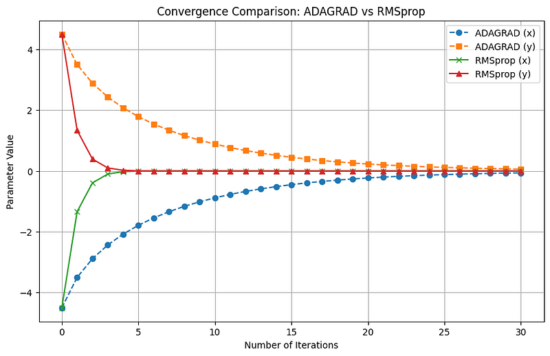
We can visualize the results:

# Plot the convergence for both methods

iterations = np.arange(num_iterations + 1)

plt.figure(figsize=(10, 6))

plt.plot(iterations, adagrad_x_values, label='ADAGRAD (x)', marker='o', linestyle='dashed')

plt.plot(iterations, adagrad_y_values, label='ADAGRAD (y)', marker='s', linestyle='dashed')

plt.plot(iterations, rmsprop_x_values, label='RMSprop (x)', marker='x')

plt.plot(iterations, rmsprop_y_values, label='RMSprop (y)', marker='^')

plt.xlabel('Number of Iterations')

plt.ylabel('Parameter Value')

plt.title('Convergence Comparison: ADAGRAD vs RMSprop')

plt.legend()

plt.grid(True)

plt.show()

As depicted, ADAGRAD's updates diminish significantly, which hinders convergence, whereas RMSprop's updates also reduce but at a more manageable pace.

Thank you for engaging with this content! If you found it helpful, consider subscribing to stay updated on future articles.

If you're interested in further reading, my book “Data-Driven Decisions: A Practical Introduction to Machine Learning” offers a comprehensive overview of machine learning concepts for just the price of a coffee. Your support is appreciated!